Solving Linear Equations

3.0 Gaussian Elimination

Last time we looked at computing the stresses in a simple truss. To solve for the
stresses, we need to solve a set of equations with several unknowns. The number of
unknowns increases as the number of elements and nodes in the truss increases. For a
very complex truss there would be many equations and unknowns.
We need a method that is very fast and can be used on a wide range of problems.
Gaussian elimination meets these requirements. It has the following attributes:

a. It works for most reasonable problems
b. It is computationally very fast
c. It is not to difficult to program

The major drawback is that it can suffer from the accumulation of round off
errors.

3.1 Upper Triangular Form (Forward Sweep)

We can illustrate how it works with the following set of equations.

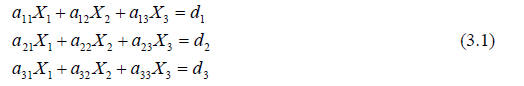
We would like to solve this set of equations for X₁ , X₂ , and X₃ . We can rewrite the
equations in matrix form as:

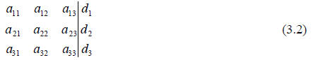
We want to multiply the first equation by some factor so that when we subtract
the second equations the a₂₁ is eliminated. We can do this by multiplying it by a₂₁ / a₁₁ .
This yields:

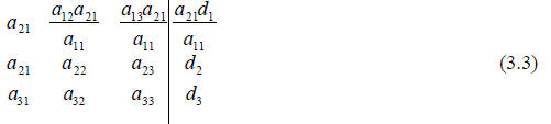
Subtracting the first equation in 3.3 from the second equation in 3.3 then replacing the
first equation with its original form yields:

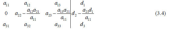
We do the same thing for the third row by multiplying the first row by a₃₁ / a₁₁
and subtracting it from the third row.

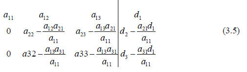
We can reduce the complexity of the terms symbolically by substituting new
variable names for the complex terms. This yields

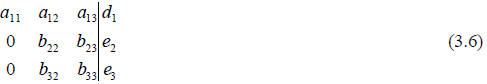
Now multiply the second row by b₃₂/b₂₂ and subtracting it from the third row.

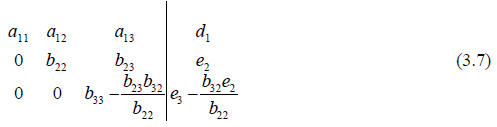
Again we simplify by substituting in for the complex terms.

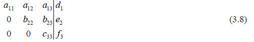
This is what we call upper triangular form. We started at the first equation and
worked our way to the last equation in what is called a forward sweep. The forward
sweep results in a matrix with values on the diagonal and above and zeros below the
diagonal.

3.2 Backward Sweep

We can solve each equation of the upper triangular form by moving through the
list starting with the bottom equation and working our way up to the top.

This is called back substitution and the process as a whole is called the backward
sweep.

3.3 Equation Normalization

You can see from the equations that it is very important for the diagonal
coefficients to be non- zero. A zero valued diagonal term will lead to a divide by zero
error.

In fact, there will be fewer problems with accumulated round off error if the
diagonal coefficients have a larger magnitude than the off diagonal terms. The reason for
this is that computers have limited precision. If the off diagonal terms are much larger
than the diagonal term, a very large number will be created when the right-hand-side of
the equation is divided by the diagonal term. The size of this number dominates the
precision of the computer and causing smaller values to be ignored when added to the
larger value. For example, adding 1.3X10¹¹ to 94.6 in a computer that has 8 digits of
precision does results in a value of 1.3X10¹¹. The 94.6 is completely lost in the process.
This can be seen in the previous example

If a₁₁ is small compared to a₂₂ then we could end up with

Small – large

And loose the value of small (a₂₂) altogether.
This problem is solved by using two steps in the processing.

a. Normalize the rows so that the largest term in the equation is 1.
b. Swap the rows around so that the largest term in any equation occurs on
the diagonal. This is called partial pivoting.

Diagonal dominance can usually be improved by moving the rows or the columns
in the set of equations. Moving the columns is somewhat more difficult than moving the
rows because the position of X₁, X₂, … changes when you move the columns. If you
move the columns you must keep track of the change in position of the Xs. When the
rows are moved, the Xs stay in the same place so rows can be moved with the added
complication.

Moving both rows and columns is called full pivoting and it is the best method for
achieving diagonal dominance. We are going to look at partial pivoting because it works
for many problems and is much simpler to implement. With partial pivoting, we are only
going to move the rows.

Before we can perform either full or partial pivoting, we must normalize the rows.
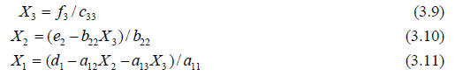
The process is illustrated in the following example. We start with the equations

We normalize each row of the equations by dividing through by the largest term in
magnitude in that row. This results in:

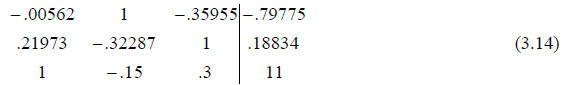
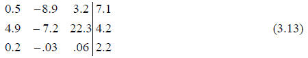
3.4 Partial Pivoting

Now we can move the equations around (partial pivoting) so that the ones are on
the diagonal. It is important to notice that normalization must be done first because
without normalization it would be difficult to know how to rearrange the equation. There
would be no basis for the row by row comparison.

These are the equations we solve using Gaussian elimination.

3.5 Overall Process

The overall process becomes
a. Normalize each equation
b. Move the equations to achieve diagonal dominance (partial pivoting).
c. Do a forward sweep that transforms the matrix to upper triangular form
d. Do a backwards sweep that solves for the values of the unknowns.

This algorithm can be written into very compact and efficient computer
algorithms and is one of the more common ways of solving large numbers of
simultaneous linear equations.

The following program reads a data file containing a matrix defining a set of
linear simultaneous linear equations. The program then executes 4 functions to solve the
system. The first function normalizes the equations, the second does partial pivoting to
achieve diagonal dominance, the third puts the matrix in upper triangular form, and the
forth function does the back substitution to solve the system of equation. The program is
sized to handle up to 100 equations and 100 unknowns.

Four functions are used to solve the equations. They are:

normal	which normalizes each row of the matrix
pivot	attempts to improve diagonal dominance by exchanging the position of rows.
forelm	the forward sweep that puts the matrix into upper triangular form
baksub	which does the back substitution to solve for the unknowns

These routines are very short and efficient.

// gauss.C - This program tests a series of routines that solve multiple
// linear equations using Gaussian elimination.

#include <fstream.h>
#include <iomanip.h>
#include <math.h>

// ROUTINES

void baksub (double a[100][100], double b[100], double x[100], int m);
void gauss (double a[100][100], double b[100], double x[100], int m);
void normal (double a[100][100], double b[100], int m);
void pivot (double a[100][100], double b[100], int m);
void forelm (double a[100][100], double b[100], int m);
void baksub (double a[100][100], double b[100], double x[100], int m);

void main (void)
{
int size, i, j;
double a[100][100], b[100], x[100];
ifstream input;

// Open the file and read the input data. The equations in the file are
// written in an augmented matrix format

input.open ("gauss.dat");
input >> size;
for (i = 0; i < size; i++)
{
for (j = 0; j < size; j++)
input >> a[i][j];
input >> b[i];
}

gauss (a, b, x, size);

// print out the results
for (i = 0; i < size; i++)
cout << "x[" << i << "] = " << x[i] << endl;
}

// Here are a series of routines that solve multiple linear equations
// using the Gaussian Elimination technique
void gauss (double a[100][100], double b[100], double x[100], int m)
{
// Normalize the matix
normal (a, b, m);
// Arrange the equations for diagonal dominance
pivot (a, b, m);
// Put into upper triangular form
forelm (a, b, m);
// Do the back substitution for the solution
baksub (a, b, x, m);
}
// This routine normalizes each row of the matrix so that the largest
// term in a row has an absolute value of one

void normal (double a[100][100], double b[100], int m)

{
int i, j;
double big;
for (i = 0; i < m; i++)
{
big = 0.0;
for (j = 0; j < m; j++)
if (big < fabs(a[i][j])) big = fabs(a[i][j]);
for (j = 0; j < m; j++)
a[i][j] = a[i][j] / big;
b[i] = b[i] / big;
}
}
// This routine attempts to rearrange the rows of the matrix so
// that the maximum value in each row occurs on the diagonal.

void pivot (double a[100][100], double b[100], int m)
{
int i, j, ibig;
double temp;
for (i = 0; i < m-1; i++)
{
ibig = i;
for (j = i+1; j < m; j++)
if (fabs (a[ibig][i]) < fabs (a[j][i])) ibig = j;
if (ibig != i)
{
for (j = 0; j < m; j++)
{
temp = a[ibig][j];
a[ibig][j] = a[i][j];
a[i][j] = temp;
}
temp = b[ibig];
b[ibig] = b[i];
b[i] = temp;
}
}
}

// This routine does the forward sweep to put the matrix in to upper
// triangular form

void forelm (double a[100][100], double b[100], int m)
{
int j, k, i;
double fact;
for (i = 0; i < m-1; i++)
{
for (j = i+1; j < m; j++)
{
if (a[i][i] != 0.0)
{
fact = a[j][i] / a[i][i];
for (k = 0; k < m; k++)
a[j][k] -= a[i][k] * fact;
b[j] -= b[i]*fact;
}
}
}
}
// This routine does the back substitution to solve the equations

void baksub (double a[100][100], double b[100], double x[100], int m)
{
int i, j;
double sum;
for (j = m-1; j >= 0; j--)
{
sum = 0.0;
for (i = j+1; i < m; i++)
sum += x[i] * a[j][i];
x[j] = (b[j] - sum) / a[j][j];
}
}