Harvey Mudd College Math Tutorial:
Solving Systems of Linear Equations; Row
Reduction

Systems of linear equations arise in all sorts of applications in many different fields of study.
The method reviewed here can be implemented to solve a linear system

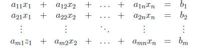
of any size. We write this system in matrix form as

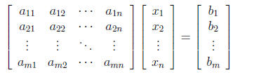
That is,
Ax = b:

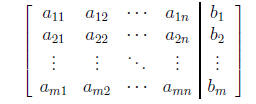
We can capture all the information contained int he sytem in the single augmented matrix

We will solve the original system of linear equations by performing a sequence of the following
elementary row operations on the augmented matrix:

Elementary Row Operations

I. Interchange two rows.
II. Multiply one row by a nonzero number.
III. Add a multiple of one row to a different row.

Do you see how we are
manipulating the system
of linear equations
by applying each of
these operations?

When a sequence of elementary row operations is performed on an augmented matrix, the
linear system that corresponds to the resulting augmented matrix is equivalent to the original
system. That is, the resulting system has the same solution set as the original system. Our

strategy in solving linear systems, therefore, is to take an augmented matrix for a system
and carry it by means of elementary row operations to an equivalent augmented matrix from
which the solutions of the system are easily obtained. In particular, we bring the augmented
matrix to Row-Echelon Form:

Row-Echelon Form

A matrix is said to be in row-echelon form if

1. All rows consisting entirely of zeros are at the bottom.
2. In each row, the first non-zero entry from the left is a 1, called the leading 1.
3. The leading 1 in each row is to the right of all leading 1's in the rows above it.

If, in addition, each leading 1 is the only non-zero entry in its column, then the matrix is in
reduced row-echelon form.

It can be proven that every matrix can be brought to row-echelon form (and even to reduced
row-echelon form) by the use of elementary row operations. At that point, the solutions of
the system are easily obtained.

In the following example, suppose that each of the matrices was the result of carrying an
augmented matrix to reduced row-echelon form by means of a sequence of row operations.

Example
The augmented matrix

in reduced row-echelon form, corresponds to the system

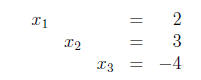
which is already fully solved!
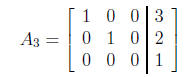
The augmented matrix

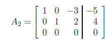
also in reduced row-echelon form, corresponds to the system

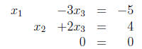
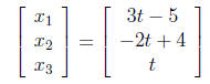
Letting x₃ = t, we find that x₂= -2t + 4 and x₁ = 3t - 5. Thus, the system has infinitely
many solutions, parametrized for all t as

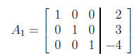
Finally, the augmented matrix

again in reduced row-echelon form, corresponds to the system

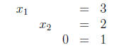
which clearly has no solution. The system is inconsistent.

Notes

If a matrix is carried to row-echelon form by means of elementary row operations, the
number of leading 1's in the resulting matrix is called the rank r of the original matrix.

Suppose that a system of linear equations in n variables has a solution. Then the set
of solutions has n - r parameters, where r is the rank of the augmented matrix.

Suppose that A is an n × n invertible matrix. Then the system Ax = b has a unique
solution given by x = A^-1b. That is, the reduced row-echelon augmented matrix will
be of the form

Gaussian Elimination

1. If the matrix is already in row-echelon form, then stop.
2. Otherwise, find the first column from the left with a non-zero entry a and move the
row containing that entry to the top of the rows being worked on.
3. Multiply that row by 1/a to create a leading 1.
4. Subtract multiples of that row from the rows below it to make each entry below the
leading 1 zero. We are now done working on that row.
5. Repeat steps 1-4 on the rows still being worked on.

Notes

In practice, you have some flexibility in the application of the algorithm. For instance,
in Step 2 you often have a choice of rows to move to the top.

A more computationally-intensive algorithm that takes a matrix to reduced row-echelon
form is given by the Gauss-Jordon Reduction.

Example
We will use Gaussian Elimination to solve the linear system

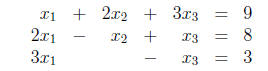
The augmented matrix is

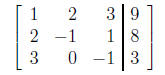
The Gaussian Elimination algorithm proceeds as follows:

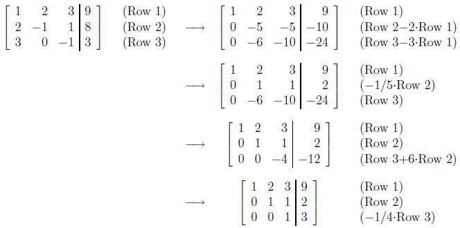
We have brought the matrix to row-echelon form. The corresponding system

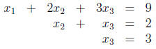
is easily solved from the bottom up:

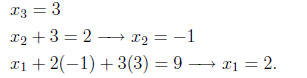
Thus, the solution of the original system is x₁ = 2; x₂ = -1; x₃ = 3:

In the Exploration, use the Row Reduction Calculator to practice solving systems of linear
equations by reducing the augmented matrices to row-echelon form.

Exploration

Key Concepts

To solve a system of linear equations, reduce the corresponding augmented matrix to row-echelon
form using the Elementary Row Operations:
I. Interchange two rows.
II. Multiply one row by a nonzero number.
III. Add a multiple of one row to a different row.

Gaussian Elimination is one algorithm that reduces matrices to row-echelon form.

[I'm ready to take the quiz.] [I need to review more.]
[Take me back to the Tutorial Page]