Solving Systems of Equations Row Reduction

Though it has not been a primary topic of interest for us, the task of
solving a system of linear equations has come up several times. For exam-
ple, if we want to show that a collection of vectors {v₁, v₂, . . . , v_k} in Rⁿ is
linearly dependent/independent, then we need to understand the solutions
(c₁, c₂, . . . , c_k) ∈ R^k of the vector equation

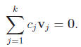
We need to keep in mind that in this equation v_j = (v_1j , v_2j , . . . , v_nj) is
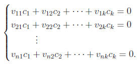
known for each j. Thus, rewriting (1) as a system, we find a system of n
equations in k unknowns:

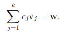
Another instance in which we have encountered systems of linear equations
is when we wanted to express a given vector w ∈ Rⁿ with respect to a given
basis, v₁, . . . , v_k. Again we seek the coefficients c₁, . . . , c₂ ∈ R of a linear
combination:

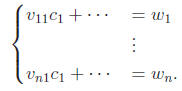
Upon converting to a system, the left side is the same as before:

When we think of these questions in terms of systems of linear equations, it
is convenient to change the names of the coefficients (the v_ij ’s and the w_j ’s)
and the unknowns c₁, . . . , c_k. First of all, let us denote the unknowns by
x = (x₁, . . . , x_k). Next we will call the coefficients of the linear terms a_ij and
the constant (affine) terms b_i, so that, after renaming, systems of the forms
(2) and (4) become

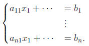
Finally, making the coefficient vectors (a_i1, . . . , a_ik) the rows of a matrix A
and thinking of the unknown x and the constant terms as column vectors,
we can write (5) in the compact form

Ax = b.

Exercise

1. Notice that (2) is simply the special case of (4) (or (3)) in which the
constant terms are zero. This special case (b = 0) is called the homogeneous
case. If b≠0, we say the system (6) is nonhomogeneous.

 (a) Show that the solution set of a homogeneous system is a subspace.
 (b) Show that the solution set of a nonhomogeneous system is an affine subspace.

(Hint: Consider the case where the system has no solution separately.)

2. (This exercise really belongs in the last set of notes, but it was left
out.) We know that the determinant of a 2 × 2 matrix gives the area
(up to a sign) of the paralellogram determined by the column vectors.
We know also that if v and w are the columns, then the parallelogram
is {av + bw : 0 ≤ a, b ≤ 1}. Give a similar interpretation for the
determinant of a 3 × 3 matrix. Be sure to precisely describe any sets
to which you refer.

As the compact form suggests, one wishes to solve (6) by simply “dividing
by” A, i.e., multiplying both sides of (6) by A^-1, so that

Such a strategy is complicated by the fact that there may be no such thing
as A^-1.

Exercise

3. What must be true about the (a) size, (b) determinant, and (c) kernel
of the associated linear transformation of the coefficient matrix A in
order for the solution (7) to make sense?

In view of the last exercise, we see that (7) represents the solution in a rather
special case. In particular, this is a case where there is exactly one solution.
In an effort to handle all the other cases, it is perhaps a good idea to consider
first simply what is likely to happen and what is possible. In all cases, let us
denote by L = R^k → Rⁿ the linear transformation associated with A.
First of all if k < n, then

dim Im(L) < n.

This means that Im(L) is a relatively thin set in Rⁿ, and (if we know nothing
else) it is unlikely that b ∈ Im(L) at all. There is most likely no solution.

Exercise

4. Given an example in which dim Im(L) < k < n and one in which
dim Im(L) = k < n. (Draw pictures.)

If there is a solution (or solutions) the question arises: How do you find it
(or them)? Another question, which is not really obvious algebraically from
(6), but is very obvious geometrically once you draw a picture is: If there is
no solution, what is the vector x which is closest to being a solution? We
will come back to this second question. Perhaps the easiest answer to the
first question (how to find solutions) is “just algebraically manipulate the
equations to solve for some of the variables in terms of the others.” Let’s
begin with an example in which k < n.

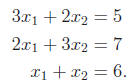
There’s no reason not to do this in an organized way. First, let us get a
coefficient of 1 in the a₁₁ position. Here we can do that by dividing the first
equation by 3. We can also accomplish our objective by putting the last
equation first:

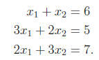
In general, you might need to do a combination of these two elementary row
operations. Next, let us use that monic coefficient to eliminate the x₁ terms
from the other equations. Multiplying the first equation by 2 and subtracting
from the last equation, we get

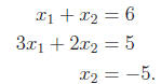
Multiplying the first equation by 3 and subtracting from the second equation:

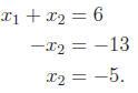
This is clearly inconsistent, i.e., there is no solution, but let us go one step
further and get a monic coefficient in the second equation

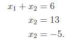
We’ll come back to this “unsolvable” system. Let’s change the constant
coefficients so that we know we have a solution

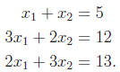
(How do you think I come up with b = (5, 12, 13)^T?) Let us also note that
there is no reason to write down the x's every time. Let us represent the
system in single matrix form:

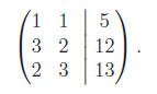
(The long vertical line is a concession to the equals signs.) Eliminating the
x₁ coefficients in the second two equations we now have

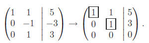
This is called Gaussian elimination and it is a convenient computational tool:
x₂ = 3, x₁ + 3 = 5 ⇒ x₁ = 2. We can also go one step further using the first
nonzero entry (pivot) in the last nonzero row to eliminate the coefficients
avove it:

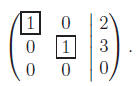
In each case, we have boxed the pivots. Let us give one more example in
which k < n.

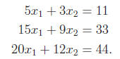
A solution via Gaussian elimination/row reduction:

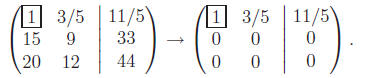
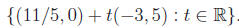
One pivot. We conclude 5x₁ + 3x₂ = 11 or x₁ = 11/5 − 3x₂/5. We can take
x₂ = t arbitrary in R to obtain the affine line of solutions

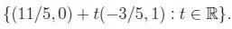
Exercise

5. Show that the solution set (8) for the last example may also be ex-
pressed as

6. Draw pictures to illustrate the three systems of equations described
above as examples.

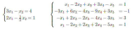
7. Describe the solution sets for the following systems of equations

(There are more systems to practice in Carlen & Carvalho pages 116–
118; 135–138.

8. The number of linearly independent rows does not change after doing
an elementary row operation.

9. The number of linearly independent columns does not change after
doing an elementary row operation.

10. The number of linearly independent rows is the number of pivots.

11. The number of linearly independent columns is the number of pivots.

12. Now can you prove the dimension theorem? Hint: How does the di-
mension of the kernel relate to the pivots?