Systems of Linear Equations and Problem Solving

SOLVING SYSTEMS OF EQUATIONS GRAPHICALLY

We can use the Intersection feature from the Math menu on the Graph screen of the TI-89 to solve a system of two equations
in two variables.

Section 8.1, Example 4(a) Solve graphically:
y − x = 1,
y + x = 3.

We graph the equations in the same viewing window and then find the coordinates of the point of intersection. Remember that
equations must be entered in “y =” form on the equation-editor screen, so we solve both equations for y. We have y = x + 1 and
y = −x + 3. Enter these equations, graph them in the standard viewing window, and find their point of intersection as described
on page 131 of this manual. We see that the solution of the system of equations is (1, 2).

MODELS
Sometimes we model two situations with linear functions and then want to find the point of intersection of their graphs.
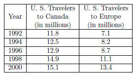
Section 8.1, Example 6 (d), (e) The numbers of U. S. travelers to Canada and to Europe are listed in the following table.

(d) Use linear regression to find two linear equations that can be used to estimate the number of U. S. travelers to Canada and
Europe, in millions, x years after 1990.

(e) Use the equations found in part (d) to estimate the year in which the number of U. S. travelers to Europe will be the same
as the number of U. S. travelers to Canada.

(d) Enter the data in the Data/Matrix editor as described on page136 of this manual. We will express the years as the number
of years since 1990 (in other words, 1990 is year 0) and enter them in c1. Then enter the number of U. S. travelers to Canada, in
millions, in c2 and the number of U. S. travelers to Europe, in millions, in c3.

Now use linear regression to fit a linear function to the data in c1 and c2. The function should also be copied to the equationeditor
screen. We will copy it as y1. See page 137 of this manual for the procedure to follow. We get y1 = 0.45x + 10.74.

Next we fit a linear function to the data in c1 and c3, enteringc1 as x and c3 as y on the Calculate screen. This function will
be copied to the equation-editor screen as y2. To enter c3 as y, position the blinkingcursor in the y box and press 3.
To select y2 as the function to which the regression equation will be copied, position the cursor beside “Store Reg EQ to,” press
, use the key to highlight y2(x) and press . We get y2 = 0.775x + 5.05.

(e) To estimate the year in which the number of U. S. travelers to Europe will be the same as the number of U. S. travelers to
Canada, we solve the system of equations
y = 0.45x + 10.74,
y = 0.775x + 5.05.

We graph the equations in the same viewing window and then use the Intersection feature to find their point of intersection.
Through a trial-and-error process we find that [0, 30, 0, 30], xscl = 2, yscl = 2, provides a good window in which to see this point.
We see that the solution of the system of equations is approximately (17.51, 18.62), so the number of U. S. travelers to Europe
will be the same as the number of U. S. travelers to Canada about 17.5 years after 1990, or in 2008.

ELIMINATION USING MATRICES

Matrices with up to 999 rows and 99 columns can be entered on the TI-89. The row-equivalent operations necessary to write a
matrix in row-echelon form or reduced row-echelon form can be performed on the calculator, or we can go directly to row-echelon
form or reduced row-echelon form with a single command. We will illustrate the direct approach for finding reduced row-echelon
form.

Section 8.6, Example 1 Solve the following system using a graphing calculator:
2x + 5y − 8z = 7,
3x + 4y − 3z = 8,
5y − 2x = 9.

First we rewrite the third equation in the form ax + by + cz = d:
2x + 5y − 8z = 7,
3x + 4y − 3z = 8,
−2x + 5y = 9.

Then we enter the coefficient matrix

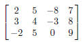
in the Data/Matrix editor. We will call the Matrix a. Press
to go to the Data/Matrix editor and set up a matrix named A with 3 rows and 4 columns. If a matrix named a has previously
been saved in your calculator, an error message will be displayed. If this happens, you can select a different name for the matrix we are about to enter or you can delete the current matrix a and then enter the new matrix as a. To delete a matrix press
to highlight the name of the matrix being deleted, and then press (VAR-LINK is the
second operation associated with the key.)

Enter the elements of the first row of the matrix by pressing 2 The cursor
moves to the element in the second row and first column of the matrix. Enter the elements of the second and third rows of the
augmented matrix by typing each in turn followed by as above. Note that the screen only displays three columns of
the matrix. The arrow keys can be used to move the cursor to any element at any time.

Matrix operations are performed on the home screen and are found on the Math Matrix menu. Press
to leave the matrix editor and go to this screen. Access the Math Matrix menu by pressing 4. (MATH is the
second operation associated with the 5 numeric key.) The reduced row-echelon form command is item 4 on this menu. Copy it to
the entry line of the home screen by pressing4. We see the command “rref(” on the entry line.

Since we want to find reduced row-echelon form for matrix a, we enter a by pressing Finally press to
see reduced row echelon form of the original matrix. We see that the solution of the system of equations isif Auto or Approximate mode is selected rather than Exact mode).

EVALUATING DETERMINANTS
We can evaluate determinants using the “det” operation from the MATRIX MATH menu.

Section 8.7, Example 3 Evaluate:

First enter the 3 x 3 matrix

as described on pages 151 and 152 of this manual. We will enter it as matrix a.

Then press to go to the home screen. Next press 4 to access the Math Matrix menu.
Press 2 to copy the “det(” operation to the entry line of the home screen. Then enter the matrix name a by pressing Finally, press to find the value of the determinant of matrix a.

INEQUALITIES IN TWO VARIABLES

The solution set of an inequality in two variables can be graphed on the TI-89.

Section 8.9, Example 4 Use a graphing calculator to graph the inequality 8x + 3y > 24.
First we write the related equation, 8x + 3y = 24, and solve it for y. We g et We will enter this as y1. Press

to go to the equation-editor screen. If there is currently an entry for y1, clear it. Also clear or deselect any other equations
that are entered. Now enter Since the inequality states that 8x + 3y > 24, or y is greater than , we want
to shade the half-plane above the graph of y₁. To do this, use the cursor to highlight y1. Then press to display the Style menu. Choose item 7, Above, by pressing7. (To shade below a line we would press 8 to select Below.) Then press 6
to see the graph of the inequality in the standard viewing window.

Note that when the “shade above” Style is selected it is not also possible to select the “Dot” style so we must keep in mind the
fact that the line is not included in the graph of the inequality. If you graphed this inequality by hand, you would
draw a dashed line.

SYSTEMS OF LINEAR INEQUALITIES

We can graph systems of inequalities by shading the solution set of each inequality in the system with a different pattern. When
the “shade above” or “shade below” style options are selected the calculator rotates through four shading patterns. Vertical lines
shade the first function, horizontal lines the second, negatively sloping diagonal lines the third, and positively sloping diagonal
lines the fourth. These patterns repeat if more than four functions are graphed.

Section 8.9, Example 8 Graph the system
x + y ≤ 4,
x −y < 4.

First graph the equation x+y = 4, enteringit in the form y = −x+4. We determine that the solution set of x+y ≤ 4 consists
of all points on or below the line x + y = 4, or y = −x + 4, so we select the “shade below” style for this function. Next graph
x − y = 4, enteringit in the form y = x − 4. The solution set of x −y < 4 is all points above the line x − y = 4, or y = x − 4, so
for this function we choose the “shade above” style. (See Example 4 above for instructions on selectingst yles.) Now press 6
to display the solution sets of each inequality in the system and the region where they overlap in the standard viewing window.
The region of overlap is the solution set of the system of inequalities. Keep in mine that the line x+y = 4, or y = −x+4, is part
of the solution set while x − y = 4, or y = x − 4, is not.